Unless you are already familiar with how to use pivot tables in Excel, you are in a way wasting what is the most powerful feature of Excel itself. I am not exaggerating here- pivot tables are the most expedient method to transform haphazard data into easily comprehensible insights without any complicated mathematical equations.
In this guide, I’ll teach you how to use pivot tables in Excel step-by-step, like a teacher—not just what to click, but why it works.
What is a Pivot Table in Excel?
You must first know what pivot tables are to learn how to use them in Excel.
A pivot table is a utility that allows you to summarize, analyze, and restructure large data sets in real time.
Rather than computing the totals, averages, or trends of a range of data by hand, pivot tables enable you to:
- Break up group data into categories.
- Calculate sums, averages, and counts
- Dynamic rearranging of rows and columns.
- Determine patterns and trends in a short time.
👉 In simple terms:
The pivot tables transform raw data into insightful reports within a few seconds.
Why You Must Learn How to Use Pivot Tables in Excel
Being frank, if you are still performing the manual calculations, then you are performing them incorrectly.
This is what happens when you get to know how to use pivot tables in Excel:
- Thousands of rows are analyzed in a second.
- You can prevent formula errors.
- You create reports within seconds, rather than hours.
- You see trends that you would not otherwise see.
Pivot tables will assist you in summarising huge datasets, contrasting values, and simply identifying patterns.
Step-by-Step: How to Use Pivot Tables in Excel
Now let’s get practical.
Step 1: Prepare Your Data
Before learning how to use pivot tables in Excel, your data must be clean.
Rules:
- Data should be in table format (rows & columns)
- No empty rows or columns
- Each column must have a header
Bad data = broken pivot table.
Step 2: Select Your Data
- Click anywhere inside your dataset
- Or select the full data range manually
This tells Excel what data to analyze.
Step 3: Insert Pivot Table
- Go to Insert → PivotTable
- Choose:
- New Worksheet (recommended)
- Or Existing Worksheet
Excel will create a blank pivot table layout.
Step 4: Understand Pivot Table Fields
This is where most beginners mess up.
When learning how to use pivot tables in Excel, you must understand these 4 areas:
- Rows → Categories (e.g., Product, Region)
- Columns → Sub-categories
- Values → Calculations (Sum, Count, Average)
- Filters → Global filters
Pivot tables work by letting you drag and drop fields into these areas.
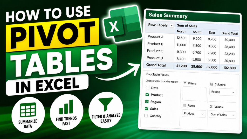
Step 5: Build Your First Pivot Table
Let’s say you have sales data.
Do this:
- Drag Product → Rows
- Drag Sales → Values
- Drag Region → Columns
Boom—you just created a report showing sales by product and region.
That’s exactly how to use pivot tables in Excel efficiently.
Example: Real Use Case
Imagine you have this data:
| Product | Region | Sales |
|---|---|---|
| Shoes | North | 1000 |
| Shoes | South | 1500 |
| Bags | North | 800 |
Using pivot tables:
- Rows → Product
- Columns → Region
- Values → Sales
You instantly get:
| Product | North | South |
|---|---|---|
| Shoes | 1000 | 1500 |
| Bags | 800 | 0 |
That’s the power of knowing how to use pivot tables in Excel.
Key Features You Must Master
If you only learn basic dragging, you’re still average. Here’s how to level up.
1. Change Value Calculation
Click on values → Value Field Settings → Choose:
- Sum
- Average
- Count
- Max/Min
Pivot tables can perform multiple calculations instantly.
2. Filter Data
Drag a field into Filters:
- Example: Filter by Region = North
- Now your report updates instantly
3. Sort Data
- Right-click → Sort
- Sort largest to smallest
This helps identify top performers quickly.
4. Group Data
You can group:
- Dates → Months / Years
- Numbers → Ranges
This makes the analysis cleaner and more readable.
5. Refresh Data
Pivot tables don’t auto-update unless you tell them.
- Right-click → Refresh
If you forget this, your analysis becomes outdated.
Also Read: Role of Artificial Intelligence in Education 2025
Try in Microsoft- Create a PivotTable to analyze worksheet data
Advanced: How to Use Pivot Tables in Excel Like a Pro
Now let’s move beyond basics.
Use Multiple Fields
You can drag multiple fields into rows:
Example:
- Region → Rows
- Product → Rows
This creates hierarchical reports.
Use Calculated Fields
You can create formulas inside pivot tables:
Example:
- Profit = Sales – Cost
No need to modify original data.
Create Pivot Charts
- Insert → Pivot Chart
This converts your pivot table into visual reports.
Use Slicers (Interactive Filters)
- Insert → Slicer
Now you can filter data with buttons.
Common Mistakes (Avoid These)
Let’s be honest—most people fail at learning how to use pivot tables in Excel because of these mistakes:
1. Bad Data Structure
If your data is messy, pivot tables won’t work properly.
2. Not Using Headers
No headers = no fields = no pivot table.
3. Forgetting Refresh
Your data changes, but the pivot table doesn’t update automatically.
4. Overcomplicating It
You don’t need formulas—pivot tables already do the heavy lifting.
Real Benefits of Using Pivot Tables
Let’s cut through the fluff.
Here’s what you actually gain when you master how to use pivot tables in Excel:
- Faster data analysis
- Better decision-making
- Reduced manual work
- Easy trend identification
- Dynamic reporting
Pivot tables allow you to summarize and reorganize data to reveal insights quickly.
When Should You Use Pivot Tables?
Use pivot tables when:
- You have large datasets
- You need quick summaries
- You want reports without formulas
- You need flexible analysis
They are especially useful for finding patterns, comparisons, and trends in data.